
Deep Learning, a term coined in 2006 refers to machine learning algorithms that have multiple non-linear layers with the ability to learn feature hierarchies. Although the basic ingredients of many deep learning algorithms have been around for many years, the advent of their popularity is owed to advances in computing power, falling cost of computing hardware, and recent advances in machine learning. Deep Neural Networks were first brought into action by Alex Krizhevsky where he used them to win the ImageNet competition(the annual Olympics of computer vision) in 2012, dropping the classification error record from 26% to 15%, an astounding improvement at the time. Since then many leading companies in the world of technology have been using deep learning networks at the core of their services. Facebook uses neural nets for their automatic tagging algorithms, Google for their photo search, Amazon for their product recommendations.
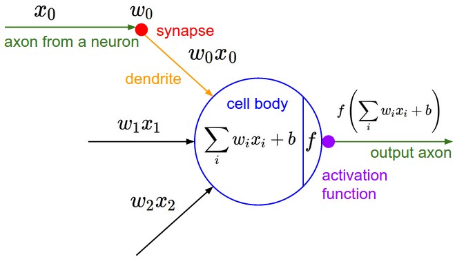
At the heart of Deep Learning Algorithms, is a Convolution Neural Network (a series of layers, each comprising of weights and biases which are learnt as part of the training process and a non-linear activation function after each layer).
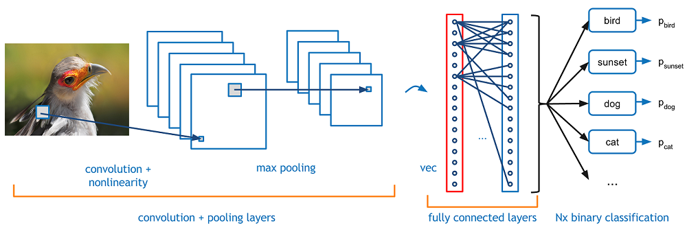
We will be using the task of Image classification (taking an input image and outputting a class (a cat, dog, etc) or a probability of classes that best describes the image) in order to understand the contribution of each layer in the decision making process of predicting whether a particular image belongs to particular class.
The Idea Behind Convolution Neural Networks
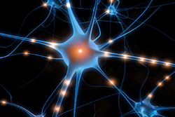
CNNs take biological inspiration from the visual cortex.The visual cortex has small regions of cells that are sensitive to specific regions of the visual field. For example, some neurons fired when exposed to vertical edges and some when shown horizontal or diagonal edges. This idea of specialized components inside of a system having specific tasks (the neuronal cells in the visual cortex looking for specific characteristics) is one that machines use as well, and is the basis behind CNNs. So every layer in a neural network can be imagined as an array of neurons with inputs from the previous layer hidden layers ( or the input layer itself) and and a non-linear activation function( eg. sigmoid, tanh, relu, selu) which processes the input to produce an output.
Input And Outputs of a CNN
For the task of image classification, the input to a CNN would be an image it has to classify. An image to a computer system is an array of pixel values. Depending upon the resolution of the image, it will see a W X H X 3 array of numbers (W: width, H: height, and 3 being the RGB values).The idea is that you give the computer this array of numbers and it will output numbers that describe the probability of the image being a certain class.
The Convolution Layer
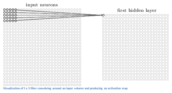
The first layer of CNN is always a convolution layer. Suppose we have an image of 32 X 32 X 3 as pixel values. The best way to contemplate a convolution layer is to image a flashlight shinning at the top left part of the image. Let’s say that the light this flashlight shines covers a 5 x 5 area. In machine learning terms, this flashlight is called a filter and the region it shines over is called the receptive field. This filter of light, is also an array of numbers called the weights. Now imagine this flashlight sliding across all areas of the input image. As the filter is sliding, it is also multiplying the weights in the filter with the original pixel values in the input image. These multiplications are then summed up to a single number. This number represents the filter output when it’s at the top left corner of the image. After sliding the filter over all the locations, you will find out that what you’re left with is a 28 x 28 x 1 array of numbers, which we call an activation map or feature map. Let’s say now we use two 5 x 5 x 3 filters instead of one. Then our output volume would be 28 x 28 x 2. By using more filters, we are able to preserve the spatial dimensions better. Mathematically, this is what’s going on in a convolutional layer.
Let’s talk about what this convolution is actually doing from a high level. Each of these filters can be thought of as low feature identifiers, each filter capturing a unique feature from the image cross-section. Now in a traditional convolutional neural network architecture, there are other layers that are interspersed between these convolution layers each having either own purpose.A classic CNN architecture would look like this.

As discussed, the the first convolution layer detects low level features such as edges, curves, colours in an image. But what happens in the case of the second convolution layer. The output of the first convolution layer acts as an input to the second convolution layer. So the input to the second conv layer is the location of low level features in the image, and when you apply the filters over it, the output will be activations that represent the presence of high level features (eg. semi-circles, squares) in the image. As you go through the network and go through more conv layers, you get activation maps that represent more and more complex features. By the end of the network, you may have some filters that activate when there is handwriting in the image, filters that activate when they see a bird’s beak, a certain colour, etc.
ReLU (Rectified Linear Units) Layers
After each convolution layer, it is convention to apply a nonlinear layer immediately afterward.The purpose of this layer is to introduce nonlinearity to a system that basically has just been computing linear operations during the convolution layers (just element wise multiplications and summations). There are other alternatives of ReLU function, such as tanh, sigmoid and bipolar sigmoid, but researchers found out that ReLU layers work far better because the network is able to train a lot faster without making a significant difference to the accuracy. It also helps to alleviate the vanishing gradient problem, which is the issue where the lower layers of the network train very slowly because the gradient decreases exponentially through the layers. It computes the function f(x)=max(0,x).
Pooling Layers
After application of a convolution layer followed by a non-linear operation (ReLU, sigmoid, tanh etc.), one may choose to downsample the output. This operation is termed as pooling. There are many operation one can perform in this layer such as max pooling, average pooling, L2-norm pooling, with max pooling being the most popular.This basically takes a filter (normally of size 2×2) and a stride of the same length. It then applies it to the input volume and outputs the maximum number in every subregion that the filter convolves around.
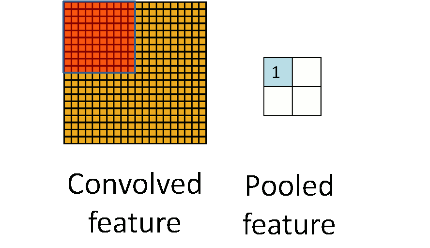
The intuitive reasoning behind this layer is that once we know that a specific feature is in the original input volume (there will be a high activation value), its exact location is not as important as its relative location to the other features. This layer serves two purposes.The first is that the amount of parameters or weights is reduced by 75%, thus lessening the computation cost. The second is that it will control overfitting.
Fully Connected Layer
Now that we can detect these high level features, the final piece of the puzzle is attaching a fully connected layer to the end of the network.This layer basically takes an input volume (whatever the output is of the convolution or ReLU or pool layer preceding it) and outputs an N dimensional vector where N is the number of classes that the program has to choose from. For example, if you wanted a digit classification program, N would be 10 since there are 10 digits. The way this fully connected layer works is that it looks at the output of the previous layer (which as we remember should represent the activation maps of high level features) and determines which features most correlate to a particular class.
Training The Network
The process of learning when it comes to humans, involves adjusting your actions for an event with prior experience in the event being used as the training set. For the case of computers, the learning process involves adjusting the filter weights and biases. The way the computer is able to adjust its filter values (or weights) is through a training process called backpropagation.
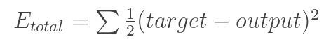
This process involves 4 stages, the forward pass, the loss function, the backward pass, and the weight update. During the forward pass, you take a training image which as we remember is a 32 x 32 x 3 array of numbers and pass it through the whole network. On our first training example, since all of the weights or filter values were randomly initialized, the output will probably be something like [.1 .1 .1 .1 .1 .1 .1 .1 .1 .1], basically an output that doesn’t give preference to any number in particular. The network, with its current weights, isn’t able to look for those low level features or thus isn’t able to make any reasonable conclusion about what the classification might be. This goes to the loss function part of backpropagation. Remember that what we are using right now is training data. This data has both an image and a label. Let’s say for example that the first training image inputted was a 3. The label for the image would be [0 0 0 1 0 0 0 0 0 0]. A loss function can be defined in many different ways but a common one is MSE (mean squared error), which is ½ times (actual – predicted) squared.
Let’s say the variable L is equal to that value. We want to get to a point where the predicted label (output of the ConvNet) is the same as the training label. In order to get there, we want to minimize the amount of loss we have. This is the mathematical equivalent of a dL/dW where W are the weights at a particular layer. Now, what we want to do is perform a backward pass through the network, which is determining which weights contributed most to the loss and finding ways to adjust them so that the loss decreases. Once we compute this derivative, we then go to the last step which is the weight update. This is where we take all the weights of the filters and update them so that they change in the opposite direction of the gradient.

Visualising the minimization of the loss
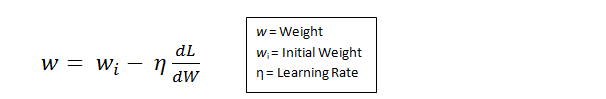
Weights Updation Process
The process of forward pass, loss function, backward pass, and parameter update is one training iteration. The program will repeat this process for a fixed number of iterations for each set of training images. Once you finish the parameter update on the last training example, hopefully the network should be trained well enough so that the weights of the layers are tuned correctly.
Deep Learning Frameworks
There are numerous deep learning frameworks such as Tensorflow (Google), Theano, Keras, Caffe, DSSTNE (Amazon), DL4J, Torch, each having it’s merits and flaws. You can explore more about these frameworks at: https://medium.com/@ricardo.guerrero/deep-learning-frameworks-a-review-before-finishing-2016-5b3ab4010b06
Here at DataMonk, we are using Tensorflow at the core of our system’s architecture to solve problems like Disease Prediction, Image Classification, Contextual chat bot to interact with Users, Building User Persona for Recommending products to users, etc. Tensorflow supports Python and C++, along to allow computing distribution among CPU, GPU (many simultaneous) and even horizontal scaling using gRPC. It’s a flexible framework supporting both low level modifications like injecting new non-linear activation to the system but also contains a high level library (tf.contrib) for people who are looking to explore the deep learning field.